Most PMs can say "LinkedIn uses ML for recommendations." Almost none can explain how the system actually works end-to-end — the layers, the trade-offs, and why it's designed that way.
That gap is what costs candidates offers at Google, Meta, and LinkedIn itself.
This article breaks down the full system in plain language. No ML PhD required.
Why This System Is Hard to Build
LinkedIn's job recommendation problem sounds simple: match people to jobs. In reality, it's three hard problems stacked on top of each other.
Problem | Scale | Why It's Hard |
|---|---|---|
Corpus size | 50M+ active job postings | Can't run a heavy model on every job for every member |
User base | 1B+ members | Preferences change daily — yesterday's signals go stale fast |
Two-sided matching | Jobs AND members both need to "match" | Relevance flows both ways — a great job for you may not want you |
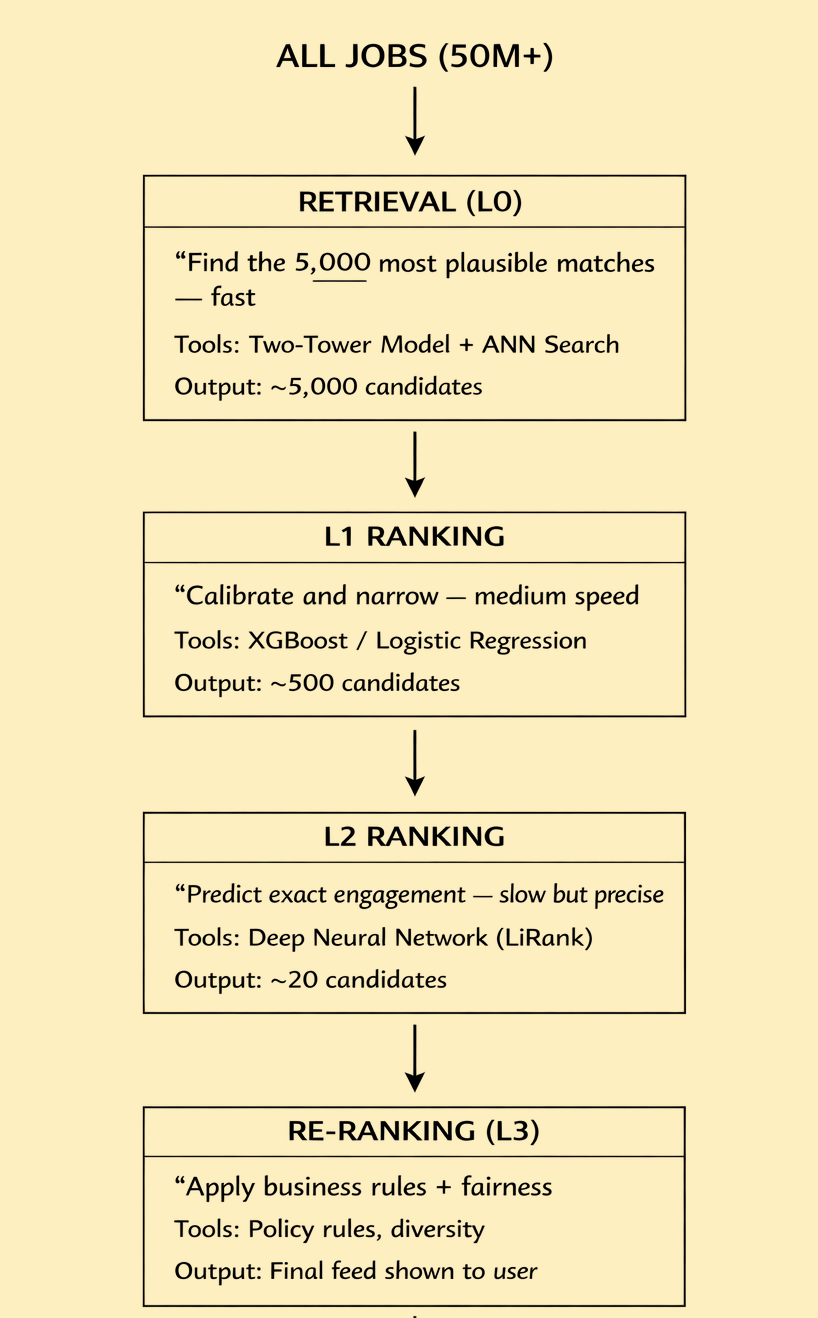
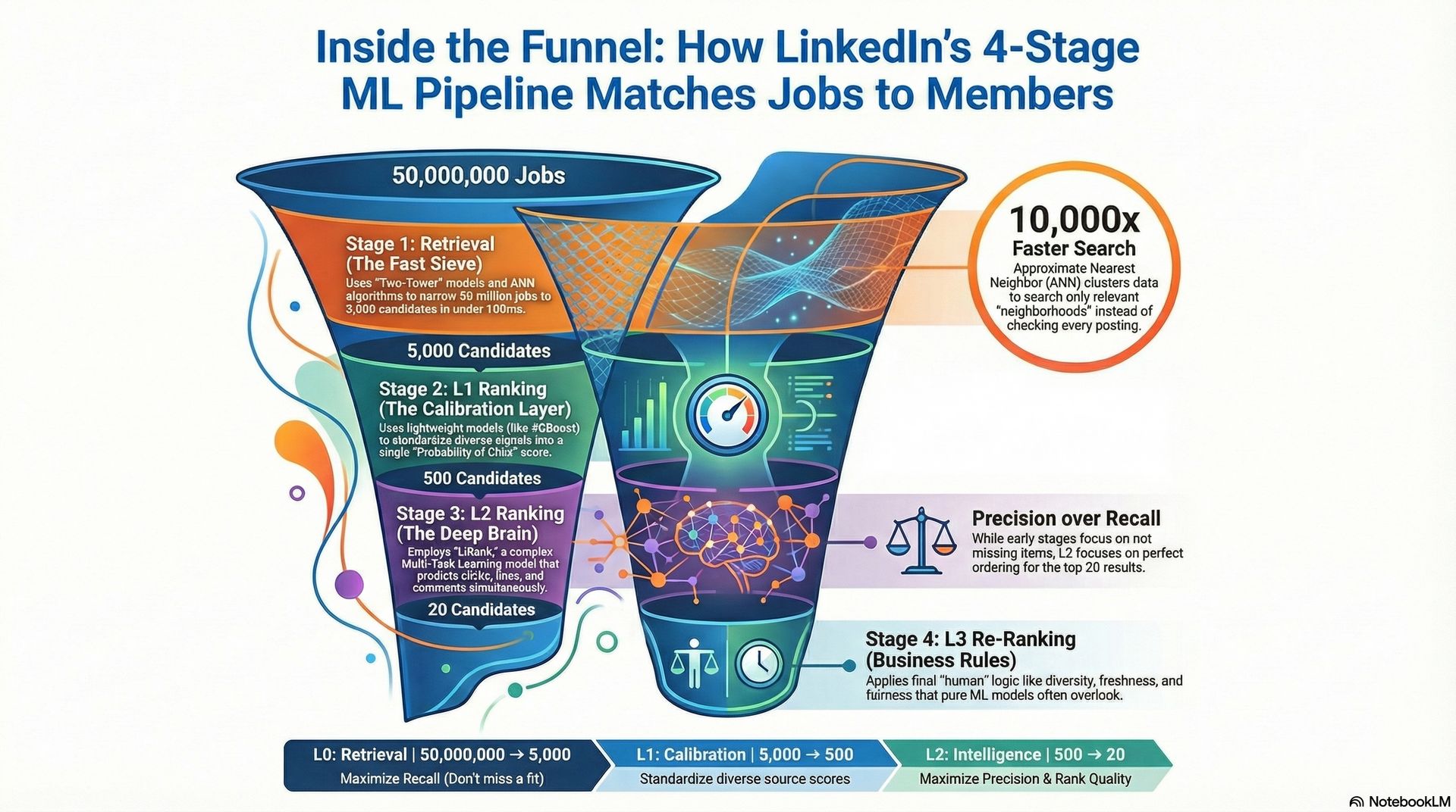
The solution is a multi-stage cascade pipeline — a funnel that gets progressively smarter and slower as it narrows down candidates.
The Full System: One Picture

High Level System Design Architecture

The rule of thumb: Each stage trades speed for intelligence. Now, we will discuss each stage in detail.
Stage 1 — Retrieval (L0): The Fast Sieve
The Job to Be Done
"From 50 million job postings, find the 5,000 that are even worth considering for this member — in under 100ms."
How It Works: Two-Tower Model + ANN
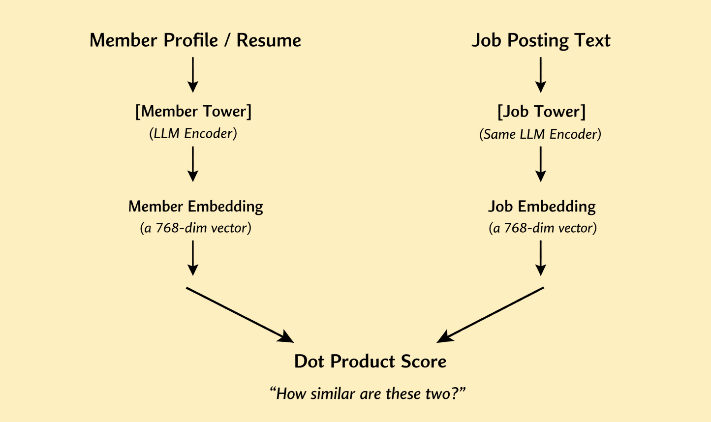
Now, lets understand the two-tier architecture. A "Two-Tower" model is a neural network designed to transform two different types of data (Users and Items) into the same mathematical space (Embeddings). Embeddings are the vector representations of the words.

The User Tower (Left Tower) has the data about the person looking at their feed. This includes their job title, skills, seniority, recent clicks, and location. The Item Tower (Right Tower) has the data about the entity being recommended (e.g., a Job Posting or a Post). This includes the job description, required skills, and the company’s industry.
The goal of the model training is to ensure that if a user is a good fit for a job, their respective vectors are "close" to each other in vector space. We measure this closeness using Cosine Similarity or a Dot Product.
The genius of Two-Tower: you pre-compute ALL job embeddings offline and store them. When a member opens LinkedIn, you only compute ONE embedding (the member's) in real-time, then do a fast similarity search against the pre-computed index.
The Search: ANN (Approximate Nearest Neighbor): Why do we need it?
Imagine LinkedIn has 20 million job postings. If a user opens their app, the system cannot calculate the "Dot Product" between the User Tower and all 20 million Item Towers in real-time. It would be too slow (high latency).
Instead of checking every single job, ANN uses clever algorithms (like HNSW or FAISS) to find the "neighborhood" where the most relevant jobs likely live.
Think of it like this:
Without ANN: Compare member embedding to all 50M jobs = 50M operations
With ANN: Partition the index into clusters, only search relevant clusters
= ~5,000 operations → 10,000x faster
How it works in production:
Offline Indexing: LinkedIn pre-calculates the embeddings for every job post and stores them in a Vector Database (like Pinecone, Milvus, or Weaviate).
Online Retrieval: When you log in, the User Tower generates your embedding.
The Search: The system asks the Vector DB: "Find me the top 5000 jobs that are mathematically closest to this user vector."
The Result: ANN returns a candidate list in a few milliseconds.
Multiple Candidate Sources
Retrieval doesn't rely on embeddings alone. The stage consists of multiple candidate generation sources — from graph-based sources that generate candidates by performing random graph walks, to embedding-based retrieval sources that generate candidates via similarity scores, to simple heuristic sources like new LinkedIn members in your geographic area.
Source Type | Example | Why It Exists |
|---|---|---|
Embedding-Based | "Your skills semantically match this role" | Catches meaning, not just keywords |
Graph-Based | "3 of your connections work at this company" | Social proof drives applications |
Heuristic | "This job is 2 miles from you" | Simple filters that are always relevant |
Collaborative Filtering | "Members like you applied to this" | Wisdom of the crowd |
These separate scouts don't talk to each other during the search. They each dump their results into a shared "bucket."
Parallel Execution: All three strategies run at the same time to save latency.
Deduplication: Since the same person might be found by both the "Graph Walk" and the "Embeddings," the system removes duplicates.
Candidate Pool (The 5,000): After deduplication, you are left with a raw list of ~5,000 people.
PM insight: Multiple retrieval sources is a product decision, not just engineering. Each source captures a different user intent. If you remove the graph-based source, you lose the "warm introduction" signal entirely.
Product Trade-offs:
Freshness vs. Latency: How often do we update the Item Tower? If a job is posted 1 minute ago, it won't be in the ANN index yet. How do we handle that? (use streaming ingestion to update a "Fresh Index" every few minutes).
Bias: If the User Tower relies too much on "Past Clicks," the user might get stuck in a "Filter Bubble." How do we introduce Exploration? (introduce a diversity re-ranker (e.g., MMR) or random "exploration" slots).
Cold Start: What do we do for a new user with zero data? The User Tower has nothing to "embed." (use demographic-based defaults or an onboarding quiz to bootstrap initial embeddings.).
Metrics at Layer 0:
Goal: Don't miss a single relevant item. High "Recall" is the priority here.
Recall@K (e.g., Recall@500): What percentage of the truly relevant items did we successfully find in our pool of 500?
Hit Rate: Did the "correct" item make it into the candidate pool at all? (Binary: Yes/No).
Latency: Since this layer scans millions of items, it must be extremely fast (usually < 20ms).
Stage 2 — L1 Ranking: The Calibration Layer
The Job to Be Done
"The 5,000 candidates came from very different sources — graph walks, embeddings, heuristics. They're not comparable yet. Calibrate them into a single ranked list and cut to 500."
Why Calibration Matters
Imagine you have two candidates:
Candidate A scored 0.92 by the embedding model
Candidate B scored 0.87 by the graph model
Which is better? You can't compare them directly — they're on different scales from different models. Because the L0 ranking has multiple candidate generation sources which could be generating very diverse candidates, calibration is an important part of this stage to make these diverse candidates comparable.
L1 job is to take raw, messy candidates from Layer 0 and turn them into a single, standardized list based on a common metric (usually Probability of Click or p(CTR)).A lightweight model like logistic regression or XGBoost could be used for calibration.
How L1 works
1. The Input: Diverse Signals
L1 receives ~5,000 candidates. For each candidate, it looks at "Signals" (Features) that L0 ignored:
The Source Signal: Which L0 scout found this person? (Graph, Embedding, or Heuristic?)
The Match Score: What was their raw score in that specific scout's system?
The Real-time Context: Is the user on a mobile phone? What time of day is it?
Simple Counters: Has this user seen this job post 3 times already today? (Frequency capping).
2. The Model: Lightweight & Fast
Because L1 still has to process 5,000 items, it cannot use a giant, "heavy" Deep Learning model. Instead, it typically uses:
Logistic Regression or LightGBM/XGBoost (Gradient Boosted Decision Trees).
Why? These models are incredibly fast at math. They can score 5,000 rows in roughly 10–20 milliseconds.
3. The Math: Scoring & Calibration
L1 doesn't care about "similarity" anymore; it cares about likelihood. It applies a weight to every signal:
Score = (w_1.EmbeddingScore) + (w_2.IsConnection) + (w_3.IsRecency)
It realizes that a "0.98 Embedding Score" is actually less valuable than a "1st-degree connection."
It "Calibrates" these into a value between 0 and 1.
4. The Output: The Top 500
Once every candidate has a calibrated score (e.g., User A = 0.85, User B = 0.42), the system:
Sorts the list from highest to lowest.
Truncates (cuts) the list. It throws away the bottom 4,500 and sends only the Top 500 to the final, most expensive Layer 2.
PM Trade-off:
Why don't we just send all 5,000 candidates straight to the final Deep Learning model (L2)?: Latency and Cost. A complex Deep Learning model takes too long to score 5,000 items. By using L1 as a 'Calibration' filter, we save ~80% of our compute cost while ensuring the final model only works on the highest-potential candidates.
Metrics at Layer 1:
Goal: Standardize different sources into a single probability.
ECE (Expected Calibration Error): Does the model's predicted probability match reality? If the model says a user has a 70% chance to click, do they actually click 70% of the time?
Log Loss: A common mathematical way to measure how "wrong" the probability predictions are.
Throughput: How many thousands of candidates can this layer process per second?
Stage 3 — L2 Ranking: The Intelligence Layer
The Job to Be Done
"From the 500 calibrated candidates, predict which 20 this specific member is most likely to apply to AND get a positive response from."
LinkedIn's L2 Model: LiRank
LinkedIn's LiRank is a large-scale ranking framework that brings to production state-of-the-art modeling architectures and optimization methods. While L1 handles "Calibration" (turning 5,000 items into 500), L2 LiRank is the "Deep Brain." It is a massive, complex Multi-Task Learning (MTL) model that performs the final, high-precision ranking.
1. The Core Architecture: Multi-Task Learning (MTL)
Instead of just predicting "Will they click?", LiRank predicts multiple outcomes simultaneously. It is essentially a "Tower of Towers."
The Click Tower: Predicts the probability of a click and "long dwell" (staying on the page).
The Contribution Tower: Predicts social actions like comments, likes, shares, and votes.
The Utility Function: LinkedIn then combines these predictions into a single final score using a weighted formula:
Score = w_1.Click + w_2.Like + w_3.Comment
Why predict multiple things? Because optimizing for clicks alone is dangerous. A clickbait job title gets applications but drives dismissals and ghosting. LinkedIn wants quality matches, not just volume.
Key Technical "Moats" of LiRank
A. Residual DCN (Deep & Cross Network)
Standard models struggle to understand complex "feature interactions" (e.g., "This user likes AI content, but only when it’s a Video posted by a 1st-degree connection").
LiRank uses Residual DCN: It adds Attention mechanisms to the feature-crossing layer. This allows the model to "pay more attention" to the specific combinations of data that actually predict a click.
B. TransAct (Sequence Modeling)
LiRank doesn't just look at who you are; it looks at what you just did.
It uses a Transformer-Encoder to look at your last 5–10 actions on LinkedIn. If you just liked three posts about "LLM Latency," LiRank will pivot your feed in real-time to show you more technical AI content, even if your "static" profile says you are interested in "General Management."
C. Isotonic Calibration Layer
Most deep learning models are "overconfident"—they might say there's a 90% chance of a click when it's really 60%.
LiRank includes a native Calibration Layer co-trained inside the neural network. This ensures that the predicted probabilities are mathematically accurate, which is vital for Ads (where LinkedIn charges based on these probabilities).
Metrics at Layer 2:
Goal: Order the items perfectly. High "Precision" and "Rank Quality" matter here.
NDCG (Normalized Discounted Cumulative Gain): Does the most relevant item appear at #1? This metric "penalizes" the system more if it puts a great job at #10 than if it puts it at #2.
MRR (Mean Reciprocal Rank): On average, how far down the list does the user have to look to find the first item they actually like?
$p(CTR)$ (Predicted Click-Through Rate): How accurate is the model at predicting user engagement?
Stage 4 — Re-Ranking (L3): Business Rules & Fairness
The Job to Be Done
"The model gave us 20 great matches. Now apply the rules that the model can't — diversity, business policy, legal fairness."
This layer is invisible in most PM interviews. It shouldn't be.
Rule Type | Example | Why It Exists |
|---|---|---|
Diversity | Don't show 20 jobs from the same company | Variety improves experience + reduces over-reliance |
Freshness | Boost jobs posted in last 48 hours | Stale listings hurt trust |
Fairness | Ensure equal exposure across demographic groups | Legal compliance + LinkedIn's values |
Business | Promote LinkedIn's hiring partners | Revenue |
Deduplication | Remove jobs the member already applied to | Basic hygiene |
Hot take: Re-ranking is where PMs have the most influence. The model gives you "technically correct." Re-ranking gives you "feels right." Those are different things.
L3 doesn't usually use a new neural network. Instead, it applies a Multiplier or a Penalty to the L2 score:
FinalScore = L2ScoreX DiversityPenalty XBusinessBoost
Metrics at Layer 3:
Goal: Balance business rules, fairness, and variety.
Diversity Score: How different are the top 10 results from each other (e.g., different industries, different media types)?
Fairness Metrics (e.g., Disparate Impact): Are we showing a representative balance of demographics (gender, race, seniority) compared to the qualified pool?
Frequency Capping: % of users who see the same item too many times (Fatigue).
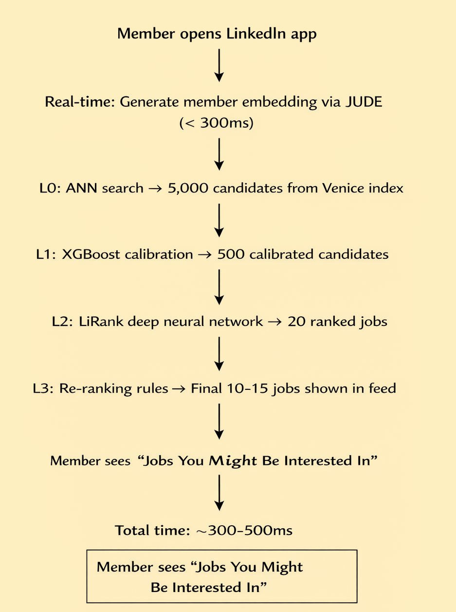
The Data Flow End-to-End

The PM-Level Trade-offs
These are the decisions that look like engineering choices but are actually product decisions.
Trade-off 1: Two-Tower vs. Cross-Encoder
Approach | Quality | Speed | Used Where |
|---|---|---|---|
Two-Tower | Good | ⚡ Fast — pre-compute one side | Retrieval + L2 features |
Cross-Encoder | Better | 🐢 Slow — must run on every pair | Not used at scale |
LinkedIn actually trained a cross-encoder to teach the two-tower model via distillation — getting 50% of the quality gap closed while keeping the speed. That's a PM-level decision: "We can't afford the best, so let's close the gap intelligently."
Trade-off 2: Freshness vs. Stability
Approach | Pro | Con |
|---|---|---|
Batch embeddings (daily) | Cheap, stable | Job posted today won't appear in recommendations until tomorrow |
Nearline (Kappa pipeline) | Near-real-time refresh | More infrastructure cost |
LinkedIn chose nearline for jobs because stale job listings are a trust-destroying experience. A job that's been filled for two weeks still appearing in recommendations is a product failure.
A kappa pipeline is the modern data engineering pattern that treats everything- both real time and historical data as a stream.
Trade-off 3: Optimize for What?
Metric | Problem if You Over-Optimize |
|---|---|
Click-through rate | Clickbait titles win; real fit loses |
Application volume | Members apply to wrong jobs; ghosting increases |
Qualified applications | Too conservative; member sees fewer options |
LinkedIn's answer: predict all four signals simultaneously in L2 and tune the weights. The weights are a product decision — not a model decision.
Summary
LinkedIn's recommendation system is a 4-stage funnel: retrieval narrows 50M jobs to 5,000 fast, L1 calibrates across sources, L2 predicts precise engagement using JUDE embeddings + behavioral signals, and re-ranking applies the business and fairness rules the model can't encode. Each stage exists because the previous one can't do what the next one does.

